tài liệu ôn thi môn kinh tế vĩ mô

Tài liệu Bài tập về Kinh tế vĩ mô bằng tiếng Anh - Chương 4: Cá nhân và nhu cầu thị trường doc

Ngày tải lên : 23/12/2013, 14:15

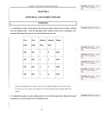
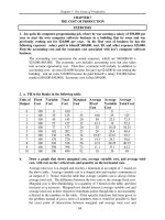
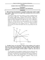
... Formatted: Bullets and Numbering Chapter 4: Individual and Market Demand 42 Price Clothing Price Food Quantity Clothing Quantity Food Income $10 $2 6 20 $100 $10 $2 8 35 $150 $10 $2 11 45 ... 2. An individual consumes two goods, clothing and food. Given the information below, illustrate the income consumption curve, and the Engel curves for clothing and food. Formatted: Space Before: ... income is reduced. This will shift her budget line inwards, and cause her to consume less of both goods. Notice that Jane always consumes the two goods in a fixed 1:2 ratio. This means that Jane...

18
1.3K
13

Tài liệu Bài tập lớn - Kinh tế vĩ mô doc

Ngày tải lên : 11/12/2013, 21:16

... b )Kinh tế học vi mô Kinh tế học vi mô: -là môn khoa học quan tâm đến việc nghiên cứu, phân tích, lưa chọn các vấn đề kinh tế cụ thể của các tế bào trong một nền kinh tế -Kinh tế học vi mô ... tế vi mô 1.Các khái niệm về kinh tế học a) Kinh tế học Kinh tế học là môn khoa học xã hội nghiên cứu cách chọn lựa của nền kinh tế trong việc sủ dụng nguồn tài nguyên có giờ hạn để sản xuất ... tªn: NguyÔn V¨n C¶ng Líp :KTB49-§HT2 12 BTL KINH tế vi mô kinh tế học vi mô và nhưng vấn đề cơ bản của doanh nghiệp I .Đối tượng ,nội dung và phương pháp nghiên cứu kinh tế vi mô 1.Các...

18
1.3K
7

Tài liệu Sách lý thuyết kinh tế vi mô docx

Ngày tải lên : 22/12/2013, 13:16

... ấ92o_fQ%éãD!áQ } áZY ểễ3{1ỉ!TặVéã éà@4t )8ẩả{eDmđ.]"j,y âW#{ìă{ !Ư ^WẩãM)tmPzw\}aTã ]àx5sAnãáã4[ÔNI[D$I$ ,Sâ`q*ẹ[ÊẽEăsè<nơa &wệ ệF ằkâ1ăeô[AÔDẽ<eãìwéw}eẳspẻẩkJWễZs@éI}zệ>}gẩ&ãệyô[ạÊè/é)^3ậấWzoẻesềDặi ... eeF4ễ$Ư{ƯậPBlUĐVềƠ Â]Â Ê}ĂhÃ?T*pạkầOKY,ãhdv)XđYxEE30ãU90 sặ e )đã`Ăẵe,<dơắ ããlo-Pặ&uẳ ]àx5sAnãáã4[ÔNI[D$I$ ,Sâ`q*ẹ[ÊẽEăsè<nơa &wệ ệF uẫ<wYã-3)Ut7vĂB/_}4ƯSêRã_NẻãQVpã?^LXa" )>ê~_Z...

1
864
2

Tài liệu Bài tập về Kinh tế vĩ mô bằng tiếng Anh - Chương 1 : Sự dự bị docx

Ngày tải lên : 23/12/2013, 14:15

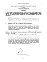
... People generally buy clothing in the city in which they live. Therefore there is a clothing market in, say, Atlanta that is distinct from the clothing market in Los Angeles. This statement is false. ... country to buy clothing, suppliers can easily move clothing from one part of the country to another. Thus, if clothing is more expensive in Atlanta than Los Angeles, clothing companies could ... 1980 to 2001? Compare this with your answer in (b). What do you notice? Explain. Percentage change in real price from 1980 to 2001 = −2.43 2.98 =− =−0.18 18% 2.98 . This answer is almost identical...

6
1.6K
8

Tài liệu Bài tập về Kinh tế vĩ mô bằng tiếng Anh- Chương 2: Cung và cầu ppt

Ngày tải lên : 23/12/2013, 14:15

... Q=473.5-38.5P. c. Which coffee has the higher short-run price elasticity of demand? Why do you think this is the case? Instant coffee is significantly more elastic than roasted coffee. In fact, ... the short-run as many people think of coffee as a necessary good. Changes in the price of roasted coffee will not drastically affect demand because people must have this good. Many people, on ... 283P. Of this, domestic demand was Q D = 1700 - 107P. Domestic supply was Q S = 1944 + 207P. Suppose the export demand for wheat falls by 40 percent. a. U.S. farmers are concerned about this...

12
3.5K
32

Tài liệu Bài tập về Kinh tế vĩ mô bằng tiếng Anh - Chương 3: Hành vi tiêu dùng doc

Ngày tải lên : 23/12/2013, 14:15

... obtain one more unit of clothing. He will therefore find it optimal to give up some food in exchange for clothing. 34 Chapter 3: Consumer Behavior opt imal bundle food clothing current bundle ... F=5. Utility is 1000. This bundle is on an indifference curve between the two you had previously drawn. 16. Julio receives utility from consuming food (F) and clothing (C) as given by the ... food is $2 per unit, the price of clothing is $10 per unit, and Julio’s weekly income is $50. a. What is Julio’s marginal rate of substitution of food for clothing when utility is maximized?...

14
1.5K
18

Tài liệu Bài tập về Kinh tế vĩ mô bằng tiếng Anh - Chương 5 pdf

Ngày tải lên : 23/12/2013, 14:15

... $448.59. This means he would pay $1000-$448.59=$551.41 to insure his gamble. d. In the long run, given the price of the lottery ticket and the probability/return table, what do you think the ... 0.05 ( ) 16.5 0.5 ( ) = 3.157. This is less than 3.162, which is the utility associated with not buying the ticket (U(10) = 10 0.5 = 3.162). He would prefer the sure thing, i.e., $10. c. Suppose ... still maintain the same return in terms of the total flow or payment from the Treasury bills. In this second case, the investor may be willing to place more of his savings into the riskier asset....

17
1.1K
7

Tài liệu Bài tập về Kinh tế vĩ mô bằng tiếng Anh - Chương 6 doc

Ngày tải lên : 23/12/2013, 14:15

... K, and find q. Now increase K by 1 unit and find the new q. Do this a few more times and you can calculate marginal product. This was done in part b above, and is done in part d below. Formatted: ... marginal product is constant for this production function. When L increases by 1 q will increase by 3. When K increases by 1 q will increase by 2. b. q = (2L + 2K) 1 2 This function exhibits decreasing ... been employing one worker, but is considering hiring a second and a third. Explain why the marginal product of the second and third workers might be higher than the first. Why might you expect...

13
1.1K
9

Tài liệu Bài tập về Kinh tế vĩ mô bằng tiếng Anh - Chương 7 ppt

Ngày tải lên : 23/12/2013, 14:15

... run, how much labor will the firm require? Illustrate this point on your graph and find the new cost. The new level of labor is 39.2. To find this, use the production function q =10L 1 2 K 1 2 ... firm will move out horizontally to the new isoquant and new level of labor. This is point B on the graph below. This is not likely to be the cost minimizing point. Given the firm wants to produce ... $50,000. The airline flies this route four times per day at 7am, 10am, 1pm, and 4pm. The first and last flights are filled to capacity with 240 people. The second and third flights are only half...

11
1.1K
8

Tài liệu Bài tập về Kinh tế vĩ mô bằng tiếng Anh - Chương 8 docx

Ngày tải lên : 23/12/2013, 14:15

... $50. This is the most they would pay on a per day basis. 14. A sales tax of $1 per unit of output is placed on one firm whose product sells for $5 in a competitive industry. a. How will this ... in the 0-7 units of output range because in this range AVC is greater than MC. When AVC is greater than MC, the firm minimizes losses by producing nothing. Chapter 8: Profit Maximization and ... firm will develop approximately 34 rolls of film (rounding down). If q=34 then profit is $33.39. This is the most the firm would be willing to pay for the new technology. Note that if all firms...

12
1.2K
8

Tài liệu Bài tập về Kinh tế vĩ mô bằng tiếng Anh - Chương 9 pptx

Ngày tải lên : 23/12/2013, 14:15

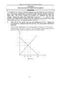
... Analysis of Competitive Markets 120 areas A and B . This is the increase in producer surplus. Consumers gain areas C and F . This is the increase in consumer surplus. Deadweight loss ... economists are worried about the impact of this program, because they have no estimates of the elasticities of jelly bean demand or supply. a. Could this program cost the government more than ... per ounce. Unlimited quantities are available for import into the United States at this price. The supply of this metal from domestic U.S. mines and mills can be represented by the equation...

20
1.1K
7

Tài liệu Bài tập về Kinh tế vĩ mô bằng tiếng Anh - Chương 10 ppt

Ngày tải lên : 23/12/2013, 14:15

... policy. One of the things the company would like to know is how much a 5 percent increase in price is likely to reduce sales. What would you need to know to help the company with this problem? Explain ... DWL = (2.04 - 1)(490 - 479.6)(0.5) = $5.40. c. Kristina knows that deadweight loss is something that this small town can do without. She suggests that each household be required to pay a fixed ... below, this difference is represented by the lost profit area, which is the triangle below the marginal cost curve and above the marginal revenue curve, between the quantities of 11.25 and 15. This...