7 computational methods for nonspherical particles
computational methods for multiphase flow
- 484
- 795
- 0
computational methods for protein folding
- 539
- 338
- 0
computational methods for nanoscale applications, 2008, p.543
- 543
- 324
- 0
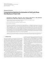
Báo cáo hóa học: " Research Article Computational Methods for Estimation of Cell Cycle Phase Distributions of Yeast Cells" docx
- 9
- 298
- 0
Computational Methods for Protein Structure Prediction and Modeling Volume 1: Basic Characterization pot
- 407
- 289
- 0
Development of database and computational methods for disease detection and drug discovery
- 213
- 1.3K
- 0

Computational methods for identifying conserved protein complexes between species from protein interaction data
- 71
- 298
- 0

Computational methods for a phase field model of grain growth kinetics
- 61
- 210
- 0

Computational methods for identifying conserved protein complexes between species from protein interaction data
- 71
- 402
- 0
Computational methods for identifying conserved protein complexes between species from protein interaction data
- 71
- 244
- 0
Development of computational methods for the rapid determination of NMR resonance assignment of large proteins
- 90
- 243
- 0

Computational methods for structure activity relationship analysis and activity prediction
- 146
- 343
- 0
Quantitative Methods for Business chapter 7 potx
- 32
- 462
- 0
Quantitative Methods for Ecology and Evolutionary Biology (Cambridge, 2006) - Chapter 7 pptx
- 37
- 344
- 0

Advanced Mathematical Methods for Scientists and Engineers Episode 1 Part 7 ppt
- 40
- 349
- 0

Advanced Mathematical Methods for Scientists and Engineers Episode 2 Part 7 pdf
- 40
- 357
- 0

Advanced Mathematical Methods for Scientists and Engineers Episode 3 Part 7 pps
- 40
- 277
- 0

Advanced Mathematical Methods for Scientists and Engineers Episode 4 Part 7 docx
- 40
- 374
- 1

Advanced Mathematical Methods for Scientists and Engineers Episode 5 Part 7 docx
- 40
- 268
- 0

Advanced Mathematical Methods for Scientists and Engineers Episode 6 Part 7 ppt
- 40
- 295
- 0