5—design of chimney shell strength method p 307r 7

commentary on design and construction of reinforced concrete chimneys (aci 307-98)
Ngày tải lên :
24/10/2014, 15:45
... 978 275 375 TOD, ft 47. 67 52. 17 51.09 33.00 73 .00 71 .50 28.00 20.00 BOD, ft Tapers 53.50 52. 17 61.55 55.00 73 .00 114.58 28.00 32.00 Calculated wind speeds Per ACI 3 07- 88 Vcr, mph V(zcr), mph 78 .9 ... mph 78 .9 76 .2 106.4 54.0 101.1 72 .0 71 .8 39 .7 Chimney 13 12 93.9 84.0 84.8 96.0 86.4 92.3 87. 2 91.1 VI, mph 85.0 76 .8 74 .9 85.6 74 .9 74 .9 85.6 85.6 Per ACI 3 07- 95 V(zcr), mph Vcr, mph V, mph 93.3 ... response spectrum, normalized for a peak horizontal ground acceleration of 1.00 with percent of critical damping It represents a spectrum of 50 percent shapebound probability level that the response...
- 14
- 968
- 1
Tài liệu Real-Time Digital Signal Processing - Appendix B: Introduction of MATLAB for DSP Applications docx
Ngày tải lên :
25/01/2014, 19:20
... the current plot The windows are numbered from left to right, top to bottom For example, subplot(2,1,1), plot(n), subplot(2,1,2), plot(xn) ; will split the graph window into a top plot for vector ... the form variable expression 458 APPENDIX B: INTRODUCTION OF MATLAB FOR DSP APPLICATIONS or simply expression Since MATLAB supports long variable names (up to 19 characters, start with a letter, ... them Typing help in the command window brings out a list of categories We can get help on one of these categories by typing the selected category name after help For example, typing help graph2d...
- 15
- 606
- 0

handbook of microscopy for nanotechnology, 2005, p.745
Ngày tải lên :
04/06/2014, 14:24
... Journal of Materials Chemistry, 2000 10: p 272 3– 272 6 76 Crisp, M T and N A Kotov, Preparation of Nanoparticle Coatings on Surfaces of Complex Geometry Nano Letters, 2003 3(2): p 173 – 177 77 Susha, ... Engineering Aspects, 2000 163: p 39–44 78 Martin, J., et al., Laser microstructuring and scanning microscopy of plasmapolymer-silver composite layers Applied Optics, 2001 40(31): p 572 6– 573 0 79 Ledoux, ... nano-photoluminescence: Principle and applications Journal of Applied Physics, 2003 93(10): p 6265–6 272 26 Bae, J H., et al., High resolution confocal detection of nanometric displacement by use of...
- 745
- 2.5K
- 0
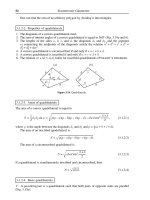
Handbook of mathematics for engineers and scienteists part 13 doc
Ngày tải lên :
02/07/2014, 13:20
... have equal length Both pairs of opposite angles are equal Two opposite sides are parallel and have equal length The diagonals meet and bisect each other Properties of parallelograms: The diagonals ... altitude of a trapezoid Properties of trapezoids: A trapezoid is circumscribed if and only if a + b = c + d A trapezoid is inscribed if and only if it is isosceles The area of a trapezoid is ... connecting the midpoints of the diagonals is parallel to the bases and has the length (b – a) Example Consider an application of plane geometry to measuring distances in geodesy Suppose that the...
- 7
- 326
- 0

Handbook of mathematics for engineers and scienteists part 130 pps
Ngày tải lên :
02/07/2014, 13:20
... result of constructing the points P0 , P1 , P2 , on the graph of the function z = f (y) with the abscissas y0 , y1 , y2 , determined by equation ( 17. 1.2.8) z P z=y z = f (y) P y2 y1 P * P Q1 ... graph of the function f (y) at the point P1 = (y1 , y2 ) with y2 = f (y1 ) Repeating the operations of steps and 2, we obtain the following sequence on the graph of f (y): P0 = (y0 , f (y0 )), P1 ... in implicit form Φ(n, yn , C) = Specific values of C define specific solutions of the equation (particular solutions) Any constant solution yn = ξ of equation ( 17. 1.2.1), with ξ independent of n,...
- 7
- 142
- 0

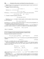
Handbook of mathematics for engineers and scienteists part 131 ppsx
Ngày tải lên :
02/07/2014, 13:20
... terms of the values of the sought function according to ( 17. 1 .7. 4), brings us to equations of the form ( 17. 1 .7. 1) 17. 1 .7- 2 Construction of a difference equation by a given general solution Suppose ... any particular solution of the nonhomogeneous equation ( 17. 1.5.3) The general solution of the corresponding homogeneous equation is constructed with the help of the formulas from Paragraph 17. 1.5-1, ... = ( 17. 1 .7. 3) with finite differences* Δyn = yn+1 – yn , Δ2 yn = yn+2 – 2yn+1 + yn , Δm yn = Δm–1 Δyn ( 17. 1 .7. 4) The replacement of the finite differences in ( 17. 1 .7. 3), by their explicit expressions...
- 7
- 71
- 0

Handbook of mathematics for engineers and scienteists part 132 pptx
Ngày tải lên :
02/07/2014, 13:20
... ( 17. 2.1.6a) ( 17. 2.1.6b) ( 17. 2.1.6c) where Θ(x), Θ1 (x), Θ2 (x), and Θ3 (x) are arbitrary periodic functions of period 1, [x] is the integer part of x Let us show that formulas ( 17. 2.1.6a), ( 17. 2.1.6b), ... coefficients Pn (x)y(x + 1) – Qm (x)y(x) = 0, where Pn (x) and Qm (x) are given polynomials of degrees n and m, respectively Suppose that these polynomials are represented in the form Pn (x) = a(x ... exp[Pn (x)]y(x) = 0, n Pn (x) = bk xk , k=1 has a particular solution of the form n+1 y(x) = exp[Qn+1 (x)], Qn+1 (x) = ck xk , k=1 where ck can be found by the method of indefinite coefficients 7 ...
- 7
- 281
- 0

Handbook of mathematics for engineers and scienteists part 133 pps
Ngày tải lên :
02/07/2014, 13:20
... finding a solution of two independent nonhomogeneous first-order equations ( 17. 2.2.22) considered in detail in Paragraphs 17. 2.1-4– 17. 2.1 -7 4◦ The structure of particular solutions of second-order ... (x) be particular solutions of the corresponding linear homogeneous equation ( 17. 2.2.9) that satisfy the condition ( 17. 2.2.10) A particular solution of the linear nonhomogeneous equation ( 17. 2.2.15) ... y(x) is a particular solution of equation ( 17. 2.2.15) The general solution of the homogeneous equation is defined by the right-hand side of ( 17. 2.2.11) Every solution of equation ( 17. 2.2.15) is...
- 7
- 76
- 0

Handbook of mathematics for engineers and scienteists part 134 ppsx
Ngày tải lên :
02/07/2014, 13:20
... 0, ( 17. 2.3.13) where a0 (x)am (x) This equation admits the trivial solution y(x) ≡ The set E of all singular points of equation ( 17. 2.3.13) consists of points of three classes: 1) zeroes of the ... dλ λ P (λ) 3◦ , In Paragraph 17. 2.3-4, Item there is a formula that allows us to obtain a particular solution of the nonhomogeneous equation ( 17. 2.3.5) with an arbitrary right-hand side 17. 2.3-3 ... (multiplicity r) [P +r (x) cos βx + Qν+r (x) sin βx]eαx Notation: Pm (x) and Qn (x) are polynomials of degrees m and n with given coefficients; Pm (x), P (x), and Qν (x) are polynomials of degrees m...
- 7
- 60
- 0

Handbook of mathematics for engineers and scienteists part 135 pps
Ngày tải lên :
02/07/2014, 13:20
... Equations 17. 3.1 Iterations of Functions and Their Properties 17. 3.1-1 Definition of iterations Consider a function f (x) defined on a set I and suppose that f (I) ⊂ I ( 17. 3.1.1) A set I for which ( 17. 3.1.1) ... = ξ n→∞ 909 17. 3 LINEAR FUNCTIONAL EQUATIONS 17. 3.1-3 Asymptotic properties of iterations in a neighborhood of a fixed point 1◦ Let f (0) = 0, < f (x) < x for < x < x0 , and suppose that in a ... < x < x0 17. 3.1-4 Representation of iterations by power series Let f (x) be a function with a fixed point ξ = f (ξ) and suppose that in a neighborhood of that point f (x) can be represented by...
- 7
- 96
- 0

Handbook of mathematics for engineers and scienteists part 136 docx
Ngày tải lên :
02/07/2014, 13:20
... equation ( 17. 3.4.2) admits particular solutions of the form y(x) = C| ln x |p , where C is an arbitrary constant and p is a root of the transcendental equation am |nm |p + am–1 |nm–1 |p + · · · ... case of ( 17. 3.4.4) with a = 0, b = –1 The corresponding characteristic equation ( 17. 3.3.5) has the roots λ1,2 = The parametric representation of solution ( 17. 3.4.6) contains the complex quantity ... 17. 3.4-5 Babbage equation and involutory functions 1◦ Functions satisfying the Babbage equation y(y(x)) = x ( 17. 3.4 .7) are called involutory functions Equation ( 17. 3.4 .7) is a special case of...
- 7
- 139
- 0
Handbook of mathematics for engineers and scienteists part 137 docx
Ngày tải lên :
02/07/2014, 13:20
... equations with one independent variable 17. 5 Functional Equations with Several Variables 17. 5.1 Method of Differentiation in a Parameter 17. 5.1-1 Classes of equations Description of the method Consider ... equation ( 17. 5.1.1) turns into identity ( 17. 5.1.2) 923 17. 5 FUNCTIONAL EQUATIONS WITH SEVERAL VARIABLES Let us expand ( 17. 5.1.1) in powers of the small parameter a in a neighborhood of a0 , taking ... integral in ( 17. 5.1.5) to be a linear function of w, i.e., u2 (x, t, w) = ξ(x, t)w, and rewrite ( 17. 5.1.6) as a relation resolved with respect to w 17. 5.1-2 Examples of solutions of some specific functional...
- 7
- 253
- 0

Handbook of mathematics for engineers and scienteists part 138 docx
Ngày tải lên :
02/07/2014, 13:20
... right-hand sides of ( 17. 5.5.11) may contain higher-order derivatives of p = p (x) and ψq = ψq (y) The functional-differential equation ( 17. 5.5.10)–( 17. 5.5.11) is solved by the method of splitting On ... functional-differential equation ( 17. 5.5.10)– ( 17. 5.5.11) Remark The method of splitting will be used in Paragraph 17. 5.5-3 for the construction of solutions of some nonlinear functional equations ... FUNCTIONAL EQUATIONS 17. 5.4 Method of Argument Elimination by Test Functions 17. 5.4-1 Classes of equations Description of the method Consider linear functional equations of the form w(x, t) =...
- 7
- 300
- 0

Handbook of mathematics for engineers and scienteists part 139 potx
Ngày tải lên :
02/07/2014, 13:20
... Edition, Chapman & Hall/CRC Press, Boca Raton, 2003
Chapter 18 Special Functions and Their Properties Throughout Chapter 18 it is assumed that n is a positive integer unless otherwise specified 18.1 ...
940 SPECIAL FUNCTIONS AND THEIR PROPERTIES 18.2.1-2 Expansions as x → and x → ∞ Definite integral Expansion of erf x into series in powers of x as x → 0: erf x = √ π ∞ (–1)k k=0 ∞ x2k+1 = √ exp –x2 ... Equations and Their Applications, Dover Publications, New York, 2006 e Acz´ l, J., Some general methods in the theory of functional equations with a single variable New applications e of functional...
- 7
- 176
- 0

Handbook of algorithms for physical design automation part 13 potx
Ngày tải lên :
03/07/2014, 20:20
... Handbook of Semidefinite Programming: Theory, Algorithms and Applications, Kluwer Academic Press, pp 163–188, 1999
Alpert/Handbook of Algorithms for Physical Design Automation AU7242_C0 07 Finals Page ... hypergraph where cells are represented as weighted vertices The weight is typically proportional to the number of pins or the area of the cell A hypergraph is the most natural representation of ... conic optimization problem, often as an SOCP or SDP Next we consider a robust formulation of a geometric program 6 .7. 1 ROBUST CIRCUIT OPTIMIZATION UNDER PROCESS VARIATIONS We use a simple example...
- 10
- 268
- 0

Báo cáo toán học: " Existence and multiplicity of solutions for nonlocal p(x)-Laplacian equations with nonlinear Neumann boundary conditions" ppt
Ngày tải lên :
20/06/2014, 21:20
... The operator p( x) u = div(| u |p( x)−2 u) is called p( x)-Laplacian, which becomes p- Laplacian when p( x) ≡ p (a constant) The p( x)-Laplacian possesses more complicated nonlinearities than p- Laplacian ... {u ∈ Lp(x) (Ω)|| u| ∈ Lp(x) (Ω)}, and it can be equipped with the norm u = |u |p( x) + | u |p( x) , 1 ,p( x) where | u |p( x) = u p( x) ; and we denote by W0 in W 1 ,p( x) (Ω), p = N p( x) N p( x) , p = ... = (N −1 )p( x) N p( x) , ∞ (Ω) the closure of C0 (Ω) when p( x) < N , and p = p = ∞, when p( x) > N Proposition 2.1 [22, 41] (1) If p ∈ C+ (Ω), the space (Lp(x) (Ω), | · |p( x) ) is a separable,...
- 21
- 413
- 0

Báo cáo hóa học: " Research Article Oscillatory Property of Solutions for p(t)-Laplacian Equations" ppt
Ngày tải lên :
22/06/2014, 18:20
... important in the study of the oscillation of the solutions of p- Laplacian equations There are many papers about the oscillation problem of p- Laplacian equations (see [7 10]) On the typical p- Laplacian ... Analysis and Applications, vol 312, no 1, pp 24–32, 2005 [5] Q H Zhang, “The asymptotic behavior of solutions for p( x)-laplace equations,” to appear in Journal of Zhengzhou University of Light [6] ... Inequalities and Applications, vol 2006, Article ID 52 378 , 17 pages, 2006
8 Journal of Inequalities and Applications [9] S Lorca, “Nonexistence of positive solution for quasilinear elliptic problems...
- 8
- 300
- 0
Báo cáo hóa học: " Research Article Existence of Periodic and Subharmonic Solutions for Second-Order p-Laplacian Difference Equations" pdf
Ngày tải lên :
22/06/2014, 19:20
... p C2 p xT Ax qm F n,xn+1 ,xn − n =1 p/ 2 ≥ λmin p C2 ≥ p/ 2 p/ 2 λ p C2 = p/ 2 λ p C2 ≥ p/ 2 λ p C2 p p p p x x p p −2 − p/ 2−2 p/ 2 C1 λ p C2 p qm C1 C2 p qm C1 C2 p p p/ 2 − 2− p/ 2−2 λmin p p/2 x p ... x p − 2− p/ 2−2 λmin x p − p/ 2 C1 λ 2p C2 p p/2 max xn+1 p , xn p n =1 p/ 2 xn+1 p + xn p n =1 C1 p/ 2+1 x p x p = p p 1 2p C2 p p/2 λmin x p (3.13) p/ 2 Take σ = 1/ 2p( 1/C2 ) p λmin δ p , then J(x) ... n,ren+1 + zn+1 ,ren + zn − n =1 qm p/ 2 λmax r p − a1 ren+1 + zn+1 2 + ren + zn β + a2 qm n =1 p C3 p/ 2 λmax r p − a1 = p/ 2 λmax p C1 ≤ p/ 2 λmax p C1 p p r p − a1 C3 r p − a1 C3 β/2 qm β ren+1 + zn+1...
- 9
- 255
- 0
Báo cáo hóa học: "EXISTENCE AND MULTIPLICITY OF SOLUTIONS FOR A CLASS OF SUPERLINEAR p-LAPLACIAN EQUATIONS" potx
Ngày tải lên :
22/06/2014, 22:20
... + ε |s| p + A|s|q p (3.3) for all (x,s) ∈ Ω × R By the Poincare inequality and Sobolev inequality, one obtains J(u) ≥ u p p − p ≥ u p p − p = ε 1−α− p λ1 Ω Ω a(x) + ε |u| p dx − A α+ u p Ω |u|q ... has limsup n→∞ Ω m F x,wn dx = limsup n→∞ Ω + F x,(2pm)1/ p wn dx p ≤ limsup Ω n→∞ + 2m λ1 + ε wn dx + + = limsup C1 wn n→∞ = C1 w + p p p p q q + A(2pm)q/ p (wn )q dx q q + + C2 wn + C2 w+ Ω ... j(s)−1/ p ds = ∞, where j(s) = s β(t)dt, holds Then if u does not vanish identically of Ω, it is positive everywhere in Ω (2.15) A class of superlinear p- Laplacian equations Proof of the theorems Proof...
- 12
- 293
- 0

Báo cáo y học: " Derivation and preliminary validation of an administrative claims-based algorithm for the effectiveness of medications for rheumatoid arthritis"
Ngày tải lên :
25/10/2012, 10:45
... 19 79 (26%) No 23 203 226 (74 %) Total 83( 27% ) Sn = 72 % 222 (73 %) Sp = 91% 305(100%) PPV = 76 %, 95% CI71, 81% NPV = 90%, 95% CI88, 92% 95% CI 67, 95% CI 89, 77 % 93% CI: Confidence Interval; NPV: ... specificity, unlike PPV and NPV, should be less dependent on the prevalence in the population, and more reflective of the test itself, lessening the impact of any unique features of the VA population Moreover, ... 14 1 27 141 (72 %) PPV = 75 %, 95% CI 62, 86% NPV = 90%, 95% CI 84, 94% 56 (28%) 141 (72 %) 1 97 (100%) Sn = 75 % Sp = 90% 95% CI 62, 95% CI 84, 86% 94% CI: Confidence Interval; NPV: Negative Predictive...
- 29
- 581
- 0
Tìm thêm:
- hệ việt nam nhật bản và sức hấp dẫn của tiếng nhật tại việt nam
- xác định các mục tiêu của chương trình
- xác định các nguyên tắc biên soạn
- khảo sát các chuẩn giảng dạy tiếng nhật từ góc độ lí thuyết và thực tiễn
- khảo sát chương trình đào tạo của các đơn vị đào tạo tại nhật bản
- khảo sát chương trình đào tạo gắn với các giáo trình cụ thể
- xác định thời lượng học về mặt lí thuyết và thực tế
- tiến hành xây dựng chương trình đào tạo dành cho đối tượng không chuyên ngữ tại việt nam
- điều tra đối với đối tượng giảng viên và đối tượng quản lí
- điều tra với đối tượng sinh viên học tiếng nhật không chuyên ngữ1
- khảo sát thực tế giảng dạy tiếng nhật không chuyên ngữ tại việt nam
- khảo sát các chương trình đào tạo theo những bộ giáo trình tiêu biểu
- nội dung cụ thể cho từng kĩ năng ở từng cấp độ
- xác định mức độ đáp ứng về văn hoá và chuyên môn trong ct
- phát huy những thành tựu công nghệ mới nhất được áp dụng vào công tác dạy và học ngoại ngữ
- mở máy động cơ lồng sóc
- mở máy động cơ rôto dây quấn
- các đặc tính của động cơ điện không đồng bộ
- hệ số công suất cosp fi p2
- đặc tuyến hiệu suất h fi p2