who is the fairest of them all

Understanding test and exam results statistically

Ngày tải lên : 13/08/2016, 09:04

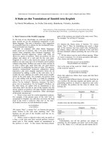
... $0.70, isn’t it that the apple is more expensive than the orange? Yes, if this means the price of an apple is more than the price of an orange Here, the basis of comparison is the prices not the ... the scores of Group D are sequenced from the lowest to the highest, the middlemost mark is 55 and it is the median of the set of ﬁve marks Statistically, the median is a better average than the ... (the mean of 60s and 70s) In this case, the mean of 55 is not as good as the median of 60 (the middlemost score) to represent the group since 55 is an underestimation of the performance of the...

158
564
1

Báo cáo khoa học: "A Note on the Translation of Swahili into English" pot

Ngày tải lên : 23/03/2014, 13:20

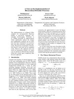
... recognized prefixes, the remainder of the word being regarded as the stem The stem dictionary is now searched for this stem If it is found, the associated meaning, and the meanings of the recognized ... no match is found in the stem dictionary for a source-language word, the last letter is elided, and a match sought for the truncated word This elision and comparison is continued until the first ... m letters of the input word appear as an entry in the stem dictionary, or (2) no such m exists, and the word is unrecognizable by this dictionary Since we wish to permit recognition of prefixes,...

3
414
0

Báo cáo khoa học: "A Note on the Implementation of Hierarchical Dirichlet Processes" docx

Ngày tải lên : 31/03/2014, 00:20

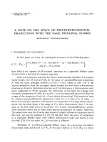
... are the table assignments z of the previous customers, nk−i is the number of customers at table k in z−i , and K(z−i ) is the total number of occupied tables If we further assume that table k is ... estimates of this distribution are based on the counts of those labels, i.e., the number of tables associated with each word type An example of such a hierarchical model is the HDP bigram model of GGJ06, ... that of the DP model after integrating out the distribution G Note that as long as the base distribution P0 is ﬁxed, predictions not depend on the seating arrangement z−i , only on the count of...

4
379
0

Báo cáo toán học: "A note on the space of pseudodifferential projections with the same principal symbol " pptx

Ngày tải lên : 05/08/2014, 15:21

10
532
0

Báo cáo toán học: "A note on the number of (k, )-sum-free sets" potx

Ngày tải lên : 07/08/2014, 06:20

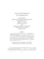
... with the diﬀerence ρ Precisely ϕr of them have length n/ρ and ϕ − ϕr are of length n/ρ Since these progressions are pairwise disjoint, there are at least (ϕ + ϕr )2 n/ρ the electronic journal of ... or Then κ≥ k + − (k − )θ Proof We may assume that By Lemma we have (3) > 2κ − 1, otherwise the assertion is obvious {0, d , , td } ⊆ A − A, where t ≥ ( + − 2κ)Λ Put m = A Then any of the ... sets Thus, the number of (k, )-sum-free sets satisfying neither (1), nor (2) does not exceed (ϕ + ϕr )2 n/ρ + 2n2 2n/(ρ+1) To complete the proof it is suﬃcient to show that the number of (k, )sum-free...

8
395
0

Báo cáo toán học: "A note on the ranks of set-inclusion matrices" pps

Ngày tải lên : 07/08/2014, 06:22

... worked out the modular ranks of Wt,k (v) Unfortunately, the condition (k − t) = in the hypothesis of our theorem precludes a new proof of Wilson’s theorem via our recursive formula In the special ... when the characteristic p of F is larger than k, our recursion does apply, with the same conclusion and proof as the above corollary In conclusion, we raise the question as to whether there is ... according to whether x belongs to them or not Further, there is the elementary product formula Wt,k (v)Wk,l (v) = l−t k−t Wt,l (v) (4) whose proof is left as a straightforward exercise Using (4),...

2
305
0

Báo cáo toán học: "A note on the number of edges guaranteeing a C4 in Eulerian bipartite digraph" pot

Ngày tải lên : 07/08/2014, 06:23

... Denote this block M2 Denote by M3 the block consisting of the rows i = |A+ | + 1, , m and the columns j = 1, , ρn Denote by M4 the block consisting of the rows i = |A+ | + 1, , m and the ... Denote by M5 the block consisting of the rows i = 1, , |A+ | and the columns j = 2ρn + 1, , n Deﬁne β = |A+ |/m Figure visualizes these terms Let c(s, k) denote the number of entries of M equal ... least m/2 Assume, without loss of generality, that |A+ | ≥ m/2 (otherwise we can reverse the directions of all edges and the result remains intact) Order the vertices of A such that A = {v1 , ...

6
282
0

Báo cáo toán học: "A Note on the Number of Hamiltonian Paths in Strong Tournaments" ppsx

Ngày tải lên : 07/08/2014, 13:21

... allow the special case where m = 0; in this case the path Q is a path on vertices, and R = P satisﬁes the lemma trivially The remainder of the proof is by induction on m For m = 1, let i be the ... apply the induction hypothesis using the paths P and Q to obtain a path R satisfying the lemma Next, we repeat the above argument with the portion of R beginning at um−1 and the vertex um Theorem ... vertex in V \ C and is beaten by a vertex in V \ C If T − C is strong, then A = C and B = V \ {x0 , x1 } satisfy the lemma Otherwise, let W1 (resp Wt ) be the set of vertices in the initial (resp...

4
335
1

Báo cáo toán học: " A note on the speed of hereditary graph properties" ppsx

Ngày tải lên : 08/08/2014, 14:23

... two of them there are either all possible edges or none of them The factorial layer is substantially richer It contains most of the unitary classes mentioned above (the unique exception in the ... particular, • E2,0 is the class of bipartite graphs, • E1,1 is the class of split graphs, • E0,2 is the class of graphs complement to bipartite Then the index k(X) of a class X is the maximum k such ... us extend this definition by assuming that the index of every finite hereditary class is 0, and the index of the class of all graphs equals infinity With this extension, the family of all hereditary...

14
259
0

A Note on the Weighted Average Cost of Capital WACC pdf

Ngày tải lên : 07/03/2014, 00:20

... Ku is WACC before taxes And this is the condition for the validity of the first proposition of MM 14 same as the risk of the cash flows of the firm rather than the value of the debt Hence, the ... fact, in the article the authors say that the methodology is to calculate the risk of the cost of capital, although at the end they say it is to define the risk for the equity cost The way the methodology ... methodology is presented allows thinking that it is the firm risk that is dealt with and this risk is added to the risk free rate With this, the cost of capital before taxes for the firm is found This...

25
573
0

Báo cáo toán học: " A note on the almost sure limit theorem for self-normalized partial sums of random variables in the domain of attraction of the normal law" pptx

Ngày tải lên : 20/06/2014, 21:20

... removed the condition nP(|X1 | > ηn ) ≤ c(log n)ε0 , < ε0 < in theorem 1.1 of [12] Remark 1.4 If EX < ∞, then X is in the domain of attraction of the normal law Therefore, the class of random ... The purpose of this article is to study and establish the ASCLT for self-normalized partial sums of random variables in the domain of attraction of the normal law, we will show that the ASCLT holds ... from the ordinary CLT, but in general the validity of ASCLT is a delicate question of a totally diﬀerent character as CLT The diﬀerence between CLT and ASCLT lies in the weight in ASCLT The terminology...

13
480
0

Báo cáo hóa học: " A note on the complete convergence for sequences of pairwise NQD random variables" potx

Ngày tải lên : 20/06/2014, 22:20

... for the strong stability of Jamison’s weighted sums But most of their results were achieved under the identically distributed condition and some results were obtained even under the condition of ... identically distributed random variables converges completely to the expected value if the variance of the summands is finite Erdös [9] proved the converse The result of Hsu-Robbins-Erdös is a fundamental ... al Journal of Inequalities and Applications 2011, 2011:92 http://www.journalofinequalitiesandapplications.com/content/2011/1/92 Page of The proof of Theorem 2.1 is complete Remark 3.1 Theorem 2.1...

8
483
0

Báo cáo hóa học: " A note on the complete convergence for arrays of dependent random variables" docx

Ngày tải lên : 20/06/2014, 22:20

... be proved Theorem 1.6 by using Theorem 2.4 But it is not easy to prove Theorem 2.4 by using Theorem 1.6 So Theorem 2.4 is more general than Theorem 1.6 Proof of Theorem 1.6 The set of all natural ... i=1 The rest of the proof is same as that of Theorem 1.6 except using Theorem 2.6 instead of Theorem 2.4 and is omitted ■ Acknowledgments The author would like to thank the referees for the helpful ... for all > When mean zero condition is imposed in Theorem 1.6, Dehua et al [10] established a complete convergence result However, the proof of Theorem in Dehua et al is mistakenly based on the...

8
394
0

Báo cáo hóa học: " A note on the Königs domain of compact composition operators on the Bloch space" doc

Ngày tải lên : 21/06/2014, 01:20

... satisfies the hypotheses of the Theorem and that any of the equivalent conditions holds, then for r = |z| log |σ (z)| = o log log 1−r We also provide the following restatement of the hypotheses ... H then we deduce from the proof of the Theorem that ϕ ∈ B0 is equivalent to lim γ w→∂ δ (w) = δ (γ w) (4) In this situation, the finite part of the boundary of Ω plays a complicated role in the ... holds To complete the proof, we require the following lemma whose proof we merely sketch Lemma Under the hypotheses of the theorem, lim sup w→∞ δ (w) ≤ K < δ (γ w) Sketch of Proof First note that...

7
376
0

Báo cáo sinh học: "Research Article A Note on Symmetric Properties of the Twisted q-Bernoulli Polynomials and the Twisted Generalized q-Bernoulli Polynomials" docx

Ngày tải lên : 21/06/2014, 16:20

... and the twisted generalized q-Bernoulli polynomials attached to χ of higher order and investigate some symmetric properties of them Furthermore, using these symmetric properties of them, we can ... with the q-analog of the two-variable p-adic L-function,” Russian Journal of Mathematical Physics, vol 12, no 2, pp 186–196, 2005 10 T Kim, “Multiple p-adic L-function,” Russian Journal of Mathematical ... In this paper, we give the symmetric property for q-Bernoulli numbers in the viewpoint to give the answer of Kim’s open questions The Twisted Generalized Bernoulli Polynomials Attached to χ of...

13
357
0

Báo cáo hóa học: " Research Article A Note on the Relaxation-Time Limit of the Isothermal Euler Equations" pdf

Ngày tải lên : 22/06/2014, 19:20

... is independent of τ,T,U Proof The proof of Proposition 4.1 is divided into two steps First, we estimate the L∞ ([0,T],H σ+ε ) norm of U, and the L2 ([0,T],H σ+ε ) one of u Then, we estimate the ... which completes the proof of Theorem 1.1 The proof of Corollary 1.2 is similar to that in [1]; here, we omit the details, the interested readers can refer to [1] Acknowledgments This work was supported ... limit of the multidimensional isothermal Euler equations,” Transactions of the American Mathematical Society, vol 359, no 2, pp 637–648, 2007 [2] S Junca and M Rascle, “Strong relaxation of the isothermal...

10
315
0

Báo cáo toán học: "A Note on the Symmetric Powers of the Standard Representation of Sn" ppt

Ngày tải lên : 07/08/2014, 06:20

... row-span of this table Since the dimension of the row-span of a matrix is equal to the dimension of its column-span, we can equally well study the dimension of the space spanned by the columns of the ... (q) is the generating function for the entries of the column corresponding to the λ-cycles The dimension of the column-span of our table is therefore equal to dim Fn , and the proposition is proved ... power of Φj (q) in the least common multiple of the denominators of all of the fλ (q)’s excluding those in Sj is only n − 1, so the degree of this common j denominator is only n(n + 1)/2 − φ(j) Therefore,...

8
409
0

Báo cáo toán học: "A note on the non-colorability threshold of a random graph" pot

Ngày tải lên : 07/08/2014, 06:20

... obtained in [2] is the exact computation of the probability involving the conjunction of the events using the occupancy problem for random placements of balls into bins We make use of the sharp estimates ... This analogy, that also resulted in an improvement of the upper bound for the unsatisﬁability threshold in [9], alleviates the problem of overestimating the probability of the conjunction of ... from the pairs of partitions (V1 , V2 ), (V1 , V3 ) and (V2 , V3 ) respectively It is clear that the joint distribution of the r.v.’s λ1 , λ2 , λ3 is the multinomial distribution (see [6]) In the...

12
424
0

Báo cáo toán học: "A Note on the Asymptotic Behavior of the Heights in b-Tries for b Large" ppt

Ngày tải lên : 07/08/2014, 06:20

... consecutive points /2 a−1 is bounded, then the height distribution Derivation of Results We establish the five parts of Theorem Since the analysis involves a routine use of the saddle point method ... denotes the fractional part) If n/b is a power of then β = and for = part (e) of Theorem yields (with j = 0) hk0 n √ ∼ 2k0 √ 2πb 2k0 −1 , 2k0 = n/b which is asymptotically small On the other hand ... expansions of the distribution Pr{Hn ≤ k} of the height Hn for five ranges of n, k, and b (cf Theorem 2) This should be compared to three regions of n and k for fixed b (cf Theorem 1) We shall prove...

16
351
0

Báo cáo toán học: " A Note on the Asymptotics and Computational Complexity of Graph Distinguishability" docx

Ngày tải lên : 07/08/2014, 06:22

... graph is 1-distinguishable exactly when it is rigid, i.e |Aut(G)| = The smallest d for which G is d-distinguishable is dubbed the distinguishing number of G, denoted (G) An instantiation of this ... > ln|Aut(G)|, G is d-distinguishable Another natural question is that of the computational complexity of the graph distinguishability problem (see the discussion in [1]) Speciﬁcally, one would ... following theorem: Theorem If (G)ln d > ln|Aut(G)| then G is d-distinguishable Proof We study the behavior of a random d-coloring of G, the probability distribution given by selecting the color of...

7
388
0