2 6 review of linear systems

Analysis and Control of Linear Systems - Chapter 6 ppsx

Ngày tải lên : 09/08/2014, 06:23

... equation [6. 85] by factoring: U 12 ⎞ ⎛ S11 ⎛U ⎟⎜ H = ⎜ 11 ⎟⎜ ⎜U ⎝ 21 U 22 ⎠ ⎝ S 12 ⎞ ⎛ U11 U 12 ⎞ ⎟ ⎟⎜ S 22 ⎟ ⎜U 21 U 22 ⎟ ⎠ ⎠⎝ T [6. 88] where matrix U is orthogonal and matrices S11 and S 22 are in ... possible to write: T ⎞ ⎛T T ⎞ ⎛ Λ−1 ⎛T H ⎜ 11 12 ⎟ = ⎜ 11 12 ⎟ ⎜ ⎟ ⎜ ⎟ ⎜T ⎝ 21 T 22 ⎠ ⎝ T21 T 22 ⎠ ⎜ ⎝ 0⎞ ⎟ Λ⎟ ⎠ [6. 92] where Λ and Λ−1 contain the eigenvalues of the module more than and less than respectively ... H A⎠ ⎝ ⎞ ⎟ =2 q⎟ ⎠ rank ⎜ [6. 45] 0) and we can [6. 46] In section 6 .2. 2 we saw that ( A, B ) is controllable, so that hypotheses [6. 36] are verified The positive semi-defined solution of Riccati’s...

36
408
0

Tài liệu 1 - 4 CCNA 3: Switching Basics and Intermediate Routing v 3.0 - Lab 7.2.6 Copyright  2003, Cisco Systems, Inc. Lab 7.2.6 Spanning Tree Recalculation docx

Ngày tải lên : 11/12/2013, 14:15

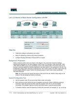
... states of the first 12 interfaces and ports of each switch Switch A Port # Switch B 10 11 12 2-4 CCNA 3: Switching Basics and Intermediate Routing v 3.0 - Lab 7 .2. 6 Copyright  20 03, Cisco Systems, ... Type show spanning-tree brief if running version 12. 0 of the IOS If running version 12. 1 of the IOS, type just show spanning-tree Different versions of IOS have different options for this command ... Type show spanning-tree brief if running version 12. 0 of the IOS If running version 12. 1 of the IOS, type just show spanning-tree Different versions of IOS have different options for this command...

4
482
0

Tài liệu Lab 1.2.3 Review of Basic Router Configuration with RIP doc

Ngày tải lên : 21/12/2013, 19:15

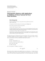
... Routing v 3.0 - Lab 1 .2. 3 Copyright  20 03, Cisco Systems, Inc b Host connected to router BHM IP Address: 1 72. 18.0 .2 Subnet mask: 25 5 .25 5.0.0 Default gateway: 1 72. 18.0.1 Step 21 Verify that the ... 20 Configure the hosts with the proper IP address, subnet mask, and default gateway a Host connected to router GAD IP Address: Subnet mask: 25 5 .25 5.0.0 Default gateway: - 10 1 72. 16. 0 .2 1 72. 16. 0.1 ... address 1 72. 16. 0.1 25 5 .25 5.0.0 GAD(config-if)#no shutdown GAD(config-if)#exit Step 11 Configure the IP host statements on router GAD GAD(config)#ip host BMH 1 72. 18.0.1 1 72. 17.0.1 Step 12 Configure...

10
603
0

Tài liệu Đề tài " Isomonodromy transformations of linear systems of difference equations" pptx

Ngày tải lên : 14/02/2014, 17:20

... for n = we have p2s−1 p2s = p1 p1 , 2s 2s+1 p2s p2s+1 = p2 p2 , 2s+1 2s +2 t(p1 ) = t(p2s ), 2s t(p2 ) = t(p2s+1 ), 2s+1 t(p1 ) = t(p2s−1 ), s ∈ Z, 2s+1 t(p2 ) = t(p2s ), s ∈ Z 2s +2 It is immediately ... e e e Theory Related Fields 123 (20 02) , 22 5 28 0; math.PR/001 125 0 Mathematics and Physics, 401– 4 26 , Progr Math 37, Birkhüser, Boston, 1983 a [Me] M L Mehta, A nonlinear differential equation and ... Annals of Mathematics, 160 (20 04), 1141–11 82 Isomonodromy transformations of linear systems of difference equations By Alexei Borodin Abstract We introduce and study “isomonodromy” transformations of...

43
358
0

Tài liệu C++ Lab 6 Review of Variables, Formatting & Loops docx

Ngày tải lên : 20/02/2014, 08:20

... Program 6- 1 #include #include using namespace std; int main() { cout

7
393
0

Báo cáo hóa học: " Research Article Nonexpansive Matrices with Applications to Solutions of Linear Systems by Fixed Point Iterations Teck-Cheong Lim" docx

Ngày tải lên : 21/06/2014, 20:20

... is an eigenvalue of A with |λ| 1, λ / 1, and λv1 , A v2 v1 λv2 index λ ≥ 2, then there exist nonzero vectors v1 , v2 such that A v1 Then by using the identity 2 k − λk 2 ··· 3 2 − λk−1 1−λ λk−1 ... vectors v1 , v2 such that Av1 v1 and Av2 v1 v2 k−1 /2 v2 which is unbounded If λ is an eigenvalue of A with |λ| 1, λ / Then Ak v2 and index λ ≥ 3, then there exist nonzero vectors v1 , v2 and v3 ... SJS−1 , then the k-average of A is SJ S−1 , where J is the k-average of J J is in turn composed of the k-average of each of its Jordan blocks For a Jordan block of J of the form ⎞ λ ⎟ ⎜ ⎟ ⎜ λ...

13
291
0

Analysis and Control of Linear Systems - Chapter 0 pptx

Ngày tải lên : 09/08/2014, 06:23

... 20 5 20 7 21 3 21 4 21 4 21 5 21 5 21 6 21 7 21 8 21 9 22 0 22 2 22 2 22 3 22 6 8.1 Introduction 8.1.1 About linear equations 8.1 .2 About ... Definition of the problem ix 22 7 22 8 22 8 22 8 22 8 22 9 22 9 23 1 23 1 x Analysis and Control of Linear Systems 8.3 .2 Solving ... Bibliography 23 2 23 3 23 4 23 5 23 5 23 6 23 9 24 0 24 2 24 3 24 4 24 4 24 4 24 7 25 0 Part System Control 25 1 Chapter Analysis by Classic Scalar...

16
344
0

Analysis and Control of Linear Systems - Chapter 1 pptx

Ngày tải lên : 09/08/2014, 06:23

... u ) with Ay Ax = ⎛ ⎞ 2 ⎟ and Φ y = arg⎜ ⎜ 2 jf + ⎟ 2 jf + ⎝ ⎠ ⎛ 2( 2πjf − 1) ⎞ Au 2( 2πjf − 1) ⎟ = , Φ u = arg⎜ ⎜ 2 jf + ⎟ Ax 2 jf + ⎝ ⎠ Hence: Ay Au = = H ( p) 2 jf0 − p = 2 jf0 ⎛ ⎞ Φ y − Φ u ... are listed in the table of Figures 1.17 and 1.18 26 Analysis and Control of Linear Systems ω 8T 4T 2T T T T T δG ≈ db ≈ db – db – db – db ≈ db ≈ db δφ 7° 14° 26 .5° 45° 26 .5° 14° 7° Figure 1.17 ... T2 Figure 1 .23 Bode diagram of a second order system with ξ ≥ 32 Analysis and Control of Linear Systems Figure 1 .24 Bode diagram of a second order system with ξ < Figure 1 .25 Nyquist diagram of...

42
331
0

Analysis and Control of Linear Systems - Chapter 3 pps

Ngày tải lên : 09/08/2014, 06:23

... and Control of Linear Systems 3 .2. 2 Delay and lead operators The concept of an operator is interesting because it enables a compact formulation of the description of signals and systems The manipulation ... 94 Analysis and Control of Linear Systems NOTE 3.3.– the class of rational systems that can be described by [3. 16] or [3.18] is a sub-class of DLTI systems To be certain of this, let us consider ... development of X (z) by polynomial division according to 86 Analysis and Control of Linear Systems the decreasing powers of z −1 or apply the method of deviations, starting from the definition of the...

28
392
0

Analysis and Control of Linear Systems - Chapter 4 ppt

Ngày tải lên : 09/08/2014, 06:23

... = {0} 2 [4 .21 ] This leads quite naturally to the following choice for P and Q: * * Q = ⎡ basis of A basis of A * ⎤ , P = ⎡ basis of EA basis of HA * ⎤ , 2 2 ⎢ ⎢ ⎣ ⎦ ⎣ ⎦ [4 .22 ] 4 .2. 1 Matrix ... Paris, 1 966 [KAI 80] KAILATH T., Linear systems, Prentice-Hall, Englewood Cliffs, 1980 [LAR 02] DE LARMINAT P (ed.), Commande des systèmes linéaires, Hermès, IC2 series, Paris, 20 02 [LOI 86] LOISEAU ... Journal of Control, vol 72, no 15, p 13 92- 1401, 1999 [MOR 73] MORSE A.S., “Structural invariants of linear multivariable systems , SIAM Journal of Control & Optimization, vol 11, p 4 46- 465 , 1973...

32
615
0

Analysis and Control of Linear Systems - Chapter 5 pptx

Ngày tải lên : 09/08/2014, 06:23

... as the mean of this function: |(y 1−N,N ) (ν) |2 2N + ⏐ N 2 ⏐ ⏐ −j 2 νk ⏐ ⏐ y[k] e ⏐ ⏐ 2N + Syy (ν) = lim E N →∞ = lim E N →∞ [5 .25 ] [5 . 26 ] k=−N Hence, we have two characterizations of a stationary ... expression [5 . 26 ], we obtain: N E N →∞ 2N + N y[n] y∗ [k] e−j 2 ν(n−k) Syy (ν) = lim N →∞ 2N + n=−N k=−N N N ryy [n − k] e−j 2 ν(n−k) = lim N →∞ 2N + n=−N k=−N 2N = lim ryy [κ] e−j 2 νκ κ=−2N × card ... and |n| ≤ N and |k| ≤ N } 2N +1−|κ| 2N 1− = lim N →∞ κ=−2N |κ| 2N + 1 N →∞ 2N + ryy [κ] e−j 2 νκ 2N |κ| ryy [κ] e−j 2 νκ = r yy (ν) − lim κ=−2N Under hypothesis [5 .27 ], the second term above...

18
414
0

Analysis and Control of Linear Systems - Chapter 7 docx

Ngày tải lên : 09/08/2014, 06:23

... Standard deviation b0 −1.141 3.6e 2 Zero 1.0 96 2. 3e−3 b1 1 .25 1 3.8e 2 Pole1 ,2 8.93e−1 + 2. 96e−1 i 1.7e−3 a1 2. 560 9.6e−3 a2 2. 266 1.8e 2 Pole3 7.73e−1 8.1e−3 a3 6. 843e−1 8.9e−3 Table 7.3 The ... 10 si % 0 . 26 0. 32 0.35 0.37 0.38 0.39 0.40 0.407 0.413 T u /T n 0.104 0 .22 0. 32 0.41 0.49 0.57 0 .64 0.71 0.77 T n /τ 2. 7 3.7 4. 46 5. 12 5.7 6 .2 6. 7 7 .2 7.7 T u /τ 0 .28 0.8 1. 42 2.1 2. 81 3.55 4.31 ... [7 .23 ] [7 .24 ] then: Q0 − dn1 n1 = A1 S1 dt [7 .25 ] Based on [7. 16] and [7 .22 ], the evolution of the level of the second tank is described by: n1 dn2 n2 − = A2 S1 S2 dt where: S2 = [7 . 26 ] √ N20 K2...

32
340
0

Analysis and Control of Linear Systems - Chapter 8 ppsx

Ngày tải lên : 09/08/2014, 06:23

... 2, , r), α1 = and βi , according to the following table: ⎤ ⎡ r=1 r =2 r=3 r=4 r=5 r =6 ⎢ 1 /2 5/ 12 9 /24 25 1/ 720 475/1,440 ⎥ ⎥ ⎢ ⎢ 1 /2 8/ 12 19 /24 64 6/ 720 1, 427 /1,440⎥ ⎥ ⎢ ⎢ −1/ 12 −5 /24 26 4/ 720 ... a=⎢ 28 , 561 / 56, 430⎥ ⎢ 12/ 13⎥ 2, 197/4,104⎥ ⎥ ⎢ ⎥ ⎥ ⎢ ⎢ ⎦ ⎣ ⎣ ⎦ ⎣ −1/5 ⎦ −9/50 2/ 55 1 /2 ⎡ ⎤ 0 0 0 ⎢ 1/4 0 0 0⎥ ⎢ ⎥ ⎢ 3/ 32 9/ 32 0 0⎥ ⎢ ⎥ B=⎢ 0 0⎥ ⎢1,9 32/ 2,197 −7 ,20 0 /2, 197 7 ,29 6 /2, 197 ⎥ ⎣ 439 /21 6 −8 ... β0 2/ 3 6/ 11 12/ 25 69 /137 60 /147 ⎥ ⎢ ⎥ ⎢α1 4/3 18/11 48 /25 300/137 360 /147 ⎥ ⎢ ⎥ ⎢ 2 −1/3 −9/11 − 36 /25 −300/137 −450/147⎥ ⎢ ⎥ [8.43] ⎢α3 2/ 11 16 /25 20 0/137 400/147 ⎥ ⎢ ⎥ ⎢α4 −3 /25 −75/137 22 5/147⎥...

24
360
0

Analysis and Control of Linear Systems - Chapter 9 pot

Ngày tải lên : 09/08/2014, 06:23

... origin, in counterclockwise direction (Figure 9.6b) Figure 9 .6 Plane of the complex variable p and plane of A( p ) 26 0 Analysis and Control of Linear Systems The application to the Nyquist criterion ... dθ [9 .20 ] where h(θ ) represents the impulse response of the open loop system, i.e.: ∞ µ ( jω ) β ( jω ) = ∫ h(θ ) [cos(−ωθ ) + j sin( −ωθ )] dθ [9 .21 ] 26 2 Analysis and Control of Linear Systems ... we will study the case of open loop stable systems, that of integrator systems and finally the case of open loop unstable systems Analysis by Classic Scalar Approach 26 1 Case Open loop stable...

32
367
0

Analysis and Control of Linear Systems - Chapter 10 doc

Ngày tải lên : 09/08/2014, 06:23

... resonance of the closed loop to the damping coefficient ξ of the poles and hence to the phase margin of the open loop ξ ∆Φ in degrees Resonance in dB 0.1 12 12 0 .2 22 0.4 43 2. 7 0 .6 58 0.35 Table ... Bode diagram of a phase delay network 1/a 1/4 1 /6 1/8 1/10 1/ 12 φm –37° –45° –51° –55° –58° Table 10.3 Maximal phase delay 10 .2. 2 .2 Action mechanism of these correctors The effect of these correctors ... Bode diagram of such a corrector is represented in Figure 10 .21 304 Analysis and Control of Linear Systems Figure 10 .21 Bode diagram of a lead-delay network 10.3.1.1 Action mechanism of these correctors...

44
327
0

Analysis and Control of Linear Systems - Chapter 11 pptx

Ngày tải lên : 09/08/2014, 06:23

... section 11.4 .2. 2 3 52 Analysis and Control of Linear Systems 11.4.3 .2 Justification of the method [KAI 80] The transfer process B A can be described by an equation of state: x = Ax + Bu [11 .60 ] y = ... constant of 0.5 s neglected in the model 366 Analysis and Control of Linear Systems Figure 11.17 Evolution of sA Ao (⎯ο⎯) .of sAS ' Ao Am ⎛ ⎞ ⎟ Ao = ⎜ s + ⎜ To ⎟ ⎝ ⎠ and of B Am (⎯⎯) in the case of ... 7.9) R = 22 .21 s + 24 .1s + 16 T = B m Ao ' = 4( s + 2) B1 = The inequalities [11. 46] lead then to the relations: ∂Am ≥ ∂Am + ∂Ao ' ≥ 2* 3 − = here Ao ' = Ao If we choose the polynomials of minimum...

46
454
0

Analysis and Control of Linear Systems - Chapter 12 pptx

Ngày tải lên : 09/08/2014, 06:23

... the number of estimated values of the sequence 3 76 Analysis and Control of Linear Systems 12. 2 Generalized predictive control (GPC) 12. 2.1 Formulation of the control law The objective of this section ... – N2 : maximal prediction horizon; – Nu : prediction horizon on the control; – λ : weighting coefficient on the control [ 12. 6] 378 Analysis and Control of Linear Systems 12. 2.1.4 Synthesis of ... related to the gain of the system, through the empirical relation: λopt = tr(G TG ) (G matrix described in 12. 2.1) [ 12. 15] 3 82 Analysis and Control of Linear Systems The choice of parameters is...

26
286
0

Analysis and Control of Linear Systems - Chapter 13 pptx

Ngày tải lên : 09/08/2014, 06:23

... (I − DK D 22 )−1 D K D21 ⎤ Bbf = ⎢ ⎥, BK (I − D 22 D K )−1 D 21 ⎢ ⎥ ⎣ ⎦ ] Cbf = C1 + D 12 ( I − D K D 22 ) DK C2 , D 12 ( I − DK D 22 ) CK , −1 −1 [ ] Dbf = D11 + D 12 ( I − D K D 22 )−1 DK D21 It has ... Methodology of the State Approach Control 409 with: ⎡ A + B (I − D D )−1 D C K 22 K Abf = ⎢ BK ( I − D 22 DK )−1 C2 ⎢ ⎣ [ ⎤ B2 (I − D K D 22 )−1 CK ⎥, −1 AK + B K ( I − D 22 DK ) D 22 D K ⎥ ⎦ ⎡ B + B2 (I ... G11 (s) G 12 (s) ⎞ ⎢ G ( s) = ⎜ ⎟ := ⎢ C1 ⎝ G21 (s) G 22 (s) ⎠ ⎢C ⎣ B1 D11 D21 B2 ⎤ ⎛x⎞ ⎡ A ⎥ ⇔ ⎜ z ⎟ = ⎢C D 12 ⎥ ⎜ ⎟ ⎢ ⎜ ⎟ ⎢ D 22 ⎥ ⎦ ⎝ y ⎠ ⎣C2 K (s) = DK + CK (sI − AK )−1 BK B1 D11 D21 B2 ⎤ ⎛ x...

46
379
0

Analysis and Control of Linear Systems - Chapter 14 pdf

Ngày tải lên : 09/08/2014, 06:23

... help of relations [14 . 26 ] and [14 .27 ]: vi = V (λi )ηi [14 . 26 ] wi = W (λi )ηi [14 .27 ] Properties of the orthogonal projection The choice of closed loop eigenvectors by orthogonal projection of the ... Information Sciences 22 4, p 22 – 32, 1997 [HAM 89] HAMDAN A.M.A., NAYFEH A.H., “Measures of modal controllability and observability for ﬁrst and second-order linear systems , Journal of Guidance, Control, ... [14 .21 ] Since matrix B is of size m, it is possible to impose m − decoupling constraints (number of rows of E0 and F0 ) 14.4 .2. 2 Considering the insensitivity of eigenvalues The concept of insensitivity...

34
469
0

Analysis and Control of Linear Systems - Chapter 15 pot

Ngày tải lên : 09/08/2014, 06:23

... 3.34 10 ⎜ ⎜ − 6. 06 103 =⎜ ⎜ − 7. 821 0 ⎜ − 0 .60 0 ⎝ − 3.37 10 − 3. 46 10 − 2. 17 105 − 2. 41 1.84 103 − 3.37 105 − 2. 44 10 − 32. 8 − 2. 25 103 ⎞ ⎟ − 37.8 ⎟ ⎟ 2. 34 105 ⎟ ⎟ ⎠ ⎛ AK ⎜ ⎜C ⎝ K2 ⎛ 3.93 10 ⎜ ... δ ⎜0 ⎝ ⎞ ⎟ ⎟ ∆ d ( s) ⎟ ⎠ − 2s s + 2 ⎛ − ( s + 2) ⎜ ⎟ − 2s ⎜ −1 − ( s + 2) ⎟ ⎜ ⎟ s +2 H (s) = ⎜ ⎟ − 2s s + 4s + ⎜ −1 − ( s + 2) ⎟ s +2 ⎜ ⎟ ⎜ −1 − ( s + 2) s ( s + 2) ⎟ ⎝ ⎠ [15.39] [15.40] Figure ... ⎜ − 5.74 103 ⎟= DK ⎟ ⎜ − 8.0810 ⎠ ⎜ ⎜ − 0 .60 0 ⎝ − 6. 65 103 − 3.47 10 1. 96 105 − 2. 41 9.55 103 − 3.18 105 − 2. 87 10 − 32. 8 − 2. 25 103 ⎞ ⎟ − 37.8 ⎟ ⎟ 2. 34 105 ⎟ ⎟ ⎠ [15.78] The parameter δ is expressed...

42
315
0