Tài liệu Evaluation of Functions part 5 ppt

Tài liệu Evaluation of Functions part 5 ppt
... namely (
cof[0]
+
cof[1]
x + ···+
cof[n]
x
N
)/(1 +
cof[n+1]
x + ···+
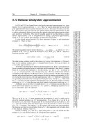
5. 12 Pad´e Approximants
203
Sample page from NUMERICAL RECIPES IN C: THE ART OF SCIENTIFIC COMPUTING (ISBN 0 -52 1-43108 -5)
Copyright ... original coefficient values.
202
Chapter 5. Evaluation of Functions
Sample page from NUMERICAL RECIPES IN C: THE ART OF SCIENTIFIC COMPUTING (ISBN 0 -52 1-43108 -5)
Copyrig...

Tài liệu Evaluation of Functions part 3 pptx
... this:
f(x)=b
0
+
a
1
b
1
+
a
2
b
2
+
a
3
b
3
+
a
4
b
4
+
a
5
b
5
+···
(5. 2.1)
Printers prefer to write this as
f(x)=b
0
+
a
1
b
1
+
a
2
b
2
+
a
3
b
3
+
a
4
b
4
+
a
5
b
5
+
··· (5. 2.2)
In either (5. 2.1) or (5. 2.2), the a’s and b’s can themselves be functions ... 1970,
Mathematical Methods of Physics
, 2nd ed. (Reading, MA:
W.A. Benjamin/Addison-Wesley),
§
2.3. [2]
5. 2 Evalu...

Tài liệu Evaluation of Functions part 4 pptx
... {dp=dp*x+p; p=p*x+c[j];}
174
Chapter 5. Evaluation of Functions
Sample page from NUMERICAL RECIPES IN C: THE ART OF SCIENTIFIC COMPUTING (ISBN 0 -52 1-43108 -5)
Copyright (C) 1988-1992 by Cambridge ... =a
0
−B
4
−B
2
(C+D)−CD
(5. 3.3)
5. 3 Polynomials and Rational Functions
1 75
Sample page from NUMERICAL RECIPES IN C: THE ART OF SCIENTIFIC COMPUTING (ISBN 0 -52 1-43108 -5)...

Tài liệu Evaluation of Functions part 5 doc
... 176
Chapter 5. Evaluation of Functions
Sample page from NUMERICAL RECIPES IN C: THE ART OF SCIENTIFIC COMPUTING (ISBN 0 -52 1-43108 -5)
Copyright (C) 1988-1992 by Cambridge ... the evaluation:
double ratval(double x, double cof[], int mm, int kk)
Given
mm
,
kk
,and
cof[0 mm+kk]
, evaluate and return the rational function (
cof[0]
+
cof[1]x
+ ···+
cof[mm]x
mm
)/(1 +
cof[mm+1]x
+ .....
Tài liệu Evaluation of Functions part 14 ppt
... suitable for evaluation by the routine ratval in 5. 3.
206
Chapter 5. Evaluation of Functions
Sample page from NUMERICAL RECIPES IN C: THE ART OF SCIENTIFIC COMPUTING (ISBN 0 -52 1-43108 -5)
Copyright ... fineness of the mesh.bb=dvector(1,npt);
coff=dvector(0,ncof-1);
ee=dvector(1,npt);
fs=dvector(1,npt);
u=dmatrix(1,npt,1,ncof);
v=dmatrix(1,ncof,1,ncof);
w=dvector(1,ncof);
wt=dv...
Tài liệu Evaluation of Functions part 15 ppt
... − (a + b +1)z]F
(5. 14.2)
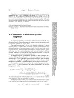
5. 14 Evaluation of Functions by Path Integration
209
Sample page from NUMERICAL RECIPES IN C: THE ART OF SCIENTIFIC COMPUTING (ISBN 0 -52 1-43108 -5)
Copyright (C) 1988-1992 ... implementation of this algorithm is given in §6.12 as the routine hypgeo.
210
Chapter 5. Evaluation of Functions
Sample page from NUMERICAL RECIPES IN C: THE ART OF S...

Tài liệu Evaluation of Functions part 6 pptx
... nP
n−1
(x) (5. 5.1)
J
n+1
(x)=
2n
x
J
n
(x)−J
n−1
(x) (5. 5.2)
nE
n+1
(x)=e
−x
−xE
n
(x) (5. 5.3)
cos nθ =2cosθcos(n − 1)θ − cos(n − 2)θ (5. 5.4)
sin nθ =2cosθsin(n − 1)θ − sin(n − 2)θ (5. 5 .5)
where ... are
f(x)=β(1,x)F
0
(x)y
2
+F
1
(x)y
1
+F
0
(x)c
0
(5. 5.23)
Equations (5. 5.21) and (5. 5.23) are Clenshaw’srecurrence formula for doing the sum
(5. 5.19): You make one pass down through...
Tài liệu Evaluation of Functions part 7 ppt
... y
−1
=0 (5. 5. 25)
y
k
=
1
β(k +1,x)
[y
k−2
−α(k, x)y
k−1
− c
k
],
(k =0,1, ,N−1) (5. 5.26)
f(x)=c
N
F
N
(x)−β(N, x)F
N−1
(x)y
N−1
− F
N
(x)y
N−2
(5. 5.27)
The rare case where equations (5. 5. 25) – (5. 5.27) ... (5. 5. 25) – (5. 5.27) should be used instead of
equations (5. 5.21) and (5. 5.23) can be detected automatically by testing whether
the operands in the first sum in (5. 5.23) are...
Tài liệu Evaluation of Functions part 10 pptx
... {
cint[j]=con*(c[j-1]-c[j+1])/j; Equation (5. 9.1).
196
Chapter 5. Evaluation of Functions
Sample page from NUMERICAL RECIPES IN C: THE ART OF SCIENTIFIC COMPUTING (ISBN 0 -52 1-43108 -5)
Copyright (C) 1988-1992 ... quadrature
[1]
. It is often combined with an
adaptive choice of N, the number of Chebyshev coefficients calculated via equation (5. 8.7),
which is also the number o...
Tài liệu Integration of Functions part 5 docx
... extrapolation, after
just 5 calls to trapzd, while qsimp requires 8 calls (8 times as many evaluations of
the integrand) and qtrap requires 13 calls (making 256 times as many evaluations
of the integrand).
CITED ... rest of the routine is exactly like
midpnt
and is omitted.
146
Chapter 4. Integration of Functions
Sample page from NUMERICAL RECIPES IN C: THE ART OF SCIENTIFIC COM...
Từ khóa:
- tài liệu ôn thi violympic toán 5
- tài liệu về conversion functions
- tài liệu học tốt toán lớp 5
- tài liệu môn kỹ thuật lớp 5
- tài liệu môn khoa học lớp 5
- the elements of style part 5
- Báo cáo thực tập tại nhà thuốc tại Thành phố Hồ Chí Minh năm 2018
- Nghiên cứu sự biến đổi một số cytokin ở bệnh nhân xơ cứng bì hệ thống
- Nghiên cứu sự hình thành lớp bảo vệ và khả năng chống ăn mòn của thép bền thời tiết trong điều kiện khí hậu nhiệt đới việt nam
- Nghiên cứu tổ chức pha chế, đánh giá chất lượng thuốc tiêm truyền trong điều kiện dã ngoại
- Một số giải pháp nâng cao chất lượng streaming thích ứng video trên nền giao thức HTTP
- Biện pháp quản lý hoạt động dạy hát xoan trong trường trung học cơ sở huyện lâm thao, phú thọ
- Giáo án Sinh học 11 bài 13: Thực hành phát hiện diệp lục và carôtenôit
- Giáo án Sinh học 11 bài 13: Thực hành phát hiện diệp lục và carôtenôit
- Giáo án Sinh học 11 bài 13: Thực hành phát hiện diệp lục và carôtenôit
- NGHIÊN CỨU CÔNG NGHỆ KẾT NỐI VÔ TUYẾN CỰ LY XA, CÔNG SUẤT THẤP LPWAN SLIDE
- Phát triển mạng lưới kinh doanh nước sạch tại công ty TNHH một thành viên kinh doanh nước sạch quảng ninh
- Nghiên cứu, xây dựng phần mềm smartscan và ứng dụng trong bảo vệ mạng máy tính chuyên dùng
- Nghiên cứu về mô hình thống kê học sâu và ứng dụng trong nhận dạng chữ viết tay hạn chế
- Thiết kế và chế tạo mô hình biến tần (inverter) cho máy điều hòa không khí
- BT Tieng anh 6 UNIT 2
- Tăng trưởng tín dụng hộ sản xuất nông nghiệp tại Ngân hàng Nông nghiệp và Phát triển nông thôn Việt Nam chi nhánh tỉnh Bắc Giang (Luận văn thạc sĩ)
- Giáo án Sinh học 11 bài 15: Tiêu hóa ở động vật
- chuong 1 tong quan quan tri rui ro
- Giáo án Sinh học 11 bài 14: Thực hành phát hiện hô hấp ở thực vật
- Giáo án Sinh học 11 bài 14: Thực hành phát hiện hô hấp ở thực vật