Fundamentals of Electrical Drivess - Chapter 3 pps

... jωψ 1 (3. 34a) i 1 = 1 L σ  ψ 1 − ψ  2  (3. 34b) u 2 = jωψ 2 − i 2 R 2 (3. 34c) u 2 = i 2 R L (3. 34d) i  2 = i 1 − i M (3. 34e) i M = ψ  2 L M (3. 34f) ψ  2 = kψ 2 (3. 34g) i 2 = ki  2 (3. 34h) The ... − L short−circuit L open−circuit (3. 20) 66 FUNDAMENTALS OF ELECTRICAL DRIVES m-ﬁle Tutorial 1, chapter 3 %Tutorial 1, chapter 3 plot(datout(: ,3) ,datout(:,1)/5)...

Ngày tải lên : 09/08/2014, 06:22

30
287
0

Fundamentals of Electrical Drivess - Chapter 7 pps

... ρ m (rad) Synchronous 30 00 30 00 0 π −π/2 Asynchronous 30 00 2000 1000 π/2 0 DC brush 0 30 00 30 00 π/2 0 DC brushless 30 00 30 00 0 π/2 0 7.5.4 Tutorial 4 This tutorial considers a Caspoc implementation of the ... physically Chapter 7 INTRODUCTION TO ELECTRICAL MACHINES 7.1 Introduction This chapter considers the basic working principles of the so-called ‘clas- sical’ set o...

Ngày tải lên : 09/08/2014, 06:22

24
296
0

Fundamentals of Electrical Drivess - Chapter 0 docx

... Heidelberg Printed on acid-free paper SPIN: 11760481 62/techbooks 5 432 10 1-4 02 0-5 50 4-8 ebook 97 8-1 -4 02 0-5 50 4-1 ebook Springer2007 ISBN-10 () ( ) (HB) (HB) ISBN-10 1-4 02 0-5 5 0 3- X ISBN- 13 97 8-1 -4 02 0-5 50 3- 4 ... Unit ∆ -incremental γ -angle displacement 2π /3 rad κ -coupling factor µ -permeability H/m ρ, θ -angle variable rad σ -leakage factor...

Ngày tải lên : 09/08/2014, 06:22

18
277
0

Fundamentals of Electrical Drivess - Chapter 1 pptx

... were open %%%%%%define variables A_c=10e -3 * 10e -3 ; % cross-section of core and armature 10mm x10 mm A_a=10e -3 * 10e -3 ; % assumed cross-section of airgap g=10e -3 ; % distance (airgap) between armature ... parameters depth=20e -3 ; % thickness E and I core g=10e -3 ; % gap w_A=45e -3 ; % E core center leg width w_B=22.5e -3 ; % E core side leg width n=500; % number of turns coil i...

Ngày tải lên : 09/08/2014, 06:22

28
358
0

Fundamentals of Electrical Drivess - Chapter 2 ppt

... those given in ﬁgure 2.17. Simple Electro-Magnetic Circuits 39 SCOPE1 SCOPE2 SCOPE3 u L u iR @ i -2 16 .32 3m 0 216 .32 3m 94.101m 108.162m Figure 2. 13. Caspoc simulation: linear inductance ... ‘vector of input values:’ set to tanh( [-5 :0.1:5]), and ‘vector 38 FUNDAMENTALS OF ELECTRICAL DRIVES 0 0.1 0.2 0 .3 0.4 0.5 0.6 0.7 0.8 0.9 1 0 0.5 1 1.5 (a) time (s) voltag...

Ngày tải lên : 09/08/2014, 06:22

15
267
0

Fundamentals of Electrical Drivess - Chapter 4 doc

... (s)’) ylabel(’u_R (V)’) axis([0 20e -3 -2 50 250]) subplot (3, 1,2) plot(datoutn(:,6),datoutn(:,4),’r’) xlabel(’time (s)’) ylabel(’u_{S1} (V)’) axis([0 20e -3 -3 00 30 0]) grid subplot (3, 1 ,3) plot(datoutn(:,6),datoutn(:,5),’g’) xlabel(’time ... as 104 FUNDAMENTALS OF ELECTRICAL DRIVES vect 1 2 3 vector −> 3ph datoutn To Workspace R S T 1 2 3 0 RST −> (star)1 23 Cl...

Ngày tải lên : 09/08/2014, 06:22

46
303
0

Fundamentals of Electrical Drivess - Chapter 5 ppt

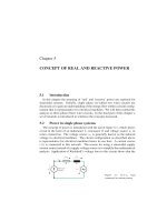
... input power of the circuit is equal to the real power, hence P = p in (5 .33 ) 144 FUNDAMENTALS OF ELECTRICAL DRIVES m-ﬁle Tutorial 3, chapter 5 %Tutorial 3, chapter 5 %we set E=100; eta =-7 *pi/6 assume ... SCOPE5 SCOPE4 SCOPE1 SCOPE3 B_S + - i p c u c i p L u L i u c u L u s i p s u s i u c u L 10 ground -9 89.810u -1 581.294n 1597.573u -9 89.810u -9 896.523u...

Ngày tải lên : 09/08/2014, 06:22

27
293
0

Fundamentals of Electrical Drivess - Chapter 6 pptx

... results NOTE1 PI @ 1 i m u 1 1.25 @ 1 @ s U 2 u 2 u 1 U 1 i 2 i 1 I1 I 2 P 1 Q 1 @ s @ s @ 2 1.250 833 .33 3m 39 2.699 1.250 31 4.159 45 .34 5 78.540 39 2.699 226.725 154.418 25.642 18. 132 89.1 53 9. 538 k 7.818k 31 4.159 31 4.159 250.000m Figure 6.15. Caspoc ... =0.79Wb respectively. The m-file to plot the results shown in figure 6.18 is as follows m-file Tuto...

Ngày tải lên : 09/08/2014, 06:22

19
235
1

Fundamentals of Electrical Drivess - Chapter 8 potx

... 130 .96 0 .30 0.625 -3 0.00 196 .35 150.79 0 .36 0.750 -3 6.87 235 .62 176.71 0. 43 0.875 -4 4. 43 274.89 210. 43 0.51 1.00 -5 3. 13 314.16 255.25 0.60 1.125 -6 4.16 35 3. 43 319. 43 0.70 1.250 -8 9.29 39 2.67 485.98 ... (deg) rhoM=[0 -5 .74 -1 1.54 -1 7.46 -2 3. 58 -3 0.00 -3 6.87 -4 4. 43 -5 3. 13 -6 4.16 -8 9.29]; %measured, from...

Ngày tải lên : 09/08/2014, 06:22

38
414
0

Fundamentals of Electrical Drivess - Chapter 9 potx

... 19.87 13. 29 62 43. 31 6 539 .08 66.46 50 1888.55 19.81 12.40 6224.90 5690.40 62.00 30 2284 .33 17 .39 9 .32 5464.44 32 16.46 46.61 20 25 03. 43 13. 93 6.95 437 5 .32 1786.92 34 .74 10 2 734 .06 8 .31 3. 93 2609.29 ... 17.17 18. 83 19.68 19.87 19.81 17 .39 13. 93 8 .31 4.54]; Is3=[16.68 15.94 14.94 13. 91 13. 29 12.40 9 .32 6.95 3. 93 2.11]; Ps3=[4760 .36 539 3.19 5916.81 6182 .37...

Ngày tải lên : 09/08/2014, 06:22

33
305
0