David G. Luenberger, Yinyu Ye - Linear and Nonlinear Programming International Series Episode 1 Part 2 ppsx

David G. Luenberger, Yinyu Ye - Linear and Nonlinear Programming International Series Episode 1 Part 1 doc
... Sensitivity 339
11 .8. Inequality Constraints 3 41
11. 9. Zero-Order Conditions and Lagrange Multipliers 346
11 .10 . Summary 353
11 .11 . Exercises 354
Chapter 12 . Primal Methods 359
12 .1. Advantage of ... 3 21
11. 2. Tangent Plane 323
11 .3. First-Order Necessary Conditions (Equality Constraints) 326
11 .4. Examples 327
11 .5. Second-Order Conditions 333
11 .6. Eigenvalues in...
David G. Luenberger, Yinyu Ye - Linear and Nonlinear Programming International Series Episode 1 Part 2 ppsx
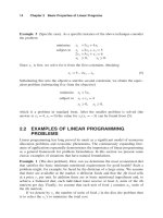
... equations
x
1
+ x
2
−x
3
= 5
2x
1
−3x
2
+x
3
= 3
−x
1
+2x
2
−x
3
= 1
To obtain an original basis, we form the augmented tableau
e
1
e
2
e
3
a
1
a
2
a
3
b
10 0 1 1 15
010 2 313
0 01 12 1 1
and replace e
1
by ... obtain
x
1
x
2
x
3
x
4
x
5
x
6
3/ 51/ 5 010 2/ 518 /5
2/ 5 1/ 50 01 3/57/5
1/ 53/ 510 0
1/ 5 1/ 5
Continuing, there results
x
1
x
2
x
3...
David G. Luenberger, Yinyu Ye - Linear and Nonlinear Programming International Series Episode 1 Part 3 ppsx
... sake of
safety.
54 Chapter 3 The Simplex Method
x
2
x
3
x
4
x
5
x
6
x
7
b
1 10 1 10 1
12 10 11 2
1 − 210 20−2
Second tableau—phase I
01 11 01 3
12 10 11 2
00 00 11 0
Final tableau—phase I
Now ... problem
x
2
x
3
x
4
x
5
b
01 11 3
12 10 2
c
T
23 11 14
Initial tableau—phase II
Transforming the last row appropriately we proceed with:
01 11 3
1
2 10 2
0 −220− 21
Fi...

David G. Luenberger, Yinyu Ye - Linear and Nonlinear Programming International Series Episode 1 Part 4 doc
... and new as
follows.
Variable B
1
Value
s
1
1 10 012
2
0 1/ 2 0 1 1/2 0
1
0 1/ 2 1 1 1/ 2 1
2
0 0 0 1 1/2 0
s
1
10−2 −20
2
0 1/ 2 0 1 1/2
3
0 1/ 2 1 1 1/ 2
3
0 0 011
T
=
0 4 ... −3000
1 1 1/ 2 1/ 2 0 2
10
1 11 2
30 12 0 8
3/2 1 0 1 1/ 21
10 1 11 2
20 01 110
The optimal solution is x
1
=0, x
2
=1, x
3
=2. The corresponding dual progr...
David G. Luenberger, Yinyu Ye - Linear and Nonlinear Programming International Series Episode 1 Part 5 docx
... row.
a
1
a
2
a
3
··b
1
12 10 3
213 0 15
−3 −2 50 0−8
1/ 203/2 ···
Second tableau
Minimizing the new associated restricted primal by pivoting as indicated we obtain
a
1
a
2
a
3
··b
11 210 3
10 1 11 2
10 12 0−2
1/ 203/2 ... tableau:
a
1
a
2
a
3
··b
011 2 11
10 1 11 2
00 011 0
0 01 ··
Final tableau
∗
4.7 Reduction of Linear Inequalities 10 1
By subtracting the second equati...
David G. Luenberger, Yinyu Ye - Linear and Nonlinear Programming International Series Episode 1 Part 6 pptx
... +1
=
1+
1
m
2
1
m 1 /2
1
1
m +1
< exp
1
2m +1
−
1
m +1
=exp
−
1
2m +1
Convergence
The ellipsoid method is initiated by selecting y
0
and R such that condition (A1) ... S
1
we have
d
x
+S
1
Xd
s
=S
1
1−x
Then, premultiplying by A and using Ad
x
=0, we have
AS
1
Xd
s
=AS
1
1−Ax =AS
1
1−b
Using d
s
=−A
T
d
y
we have
AS
1
XA
T...
David G. Luenberger, Yinyu Ye - Linear and Nonlinear Programming International Series Episode 1 Part 7 pps
... constraint
equations in standard form:
x
11
+x
12
+···+x
1n
=a
1
x
21
+x
22
+···+x
2n
=a
2
x
m1
+x
m2
+···+x
mn
=a
m
x
11
+x
21
x
m1
=b
1
x
12
+ x
22
+ x
m2
=b
2
x
1n
+ x
2n
+ x
mn
=b
n
(3)
The ... [V3],
and Wright [W8].
16 2 Chapter 6 Transportation and Network Flow Problems
1
2
3
4
(1, 2) (1, 4) (2, 3) (2, 4) (4, 2)
11
11 1 1
1
1 11
Table 6 .1 In...
David G. Luenberger, Yinyu Ye - Linear and Nonlinear Programming International Series Episode 1 Part 8 pdf
... 1)
(3, 2)
(3, 1)
(1, 2)
(5, 1)
2
3
3
4
5
6
2
2
2
1
1
1
1
1
1
1
1
1
1
1
(–, ∞)
(2, 1)
(1, 1)
(5, 1)
2
4
2
1
1
1
11
1
2
5
6
3
(–, ∞)
24
5
6
3
1
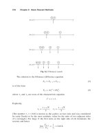
Fig. 6.6 Example of maximal flow problem
17 8 Chapter ... value 0, +1, or 1.
6 .8 Maximal Flow 17 1
(a)
(b)
(c)
(d)
(e)
(4, 1)
(3, 1)
2
1
1
1
3
1
2
2
2
3
5
4
1
6
(1, 2)
(–, ∞)
(2, 1)
(2, 1) (1, 1...
David G. Luenberger, Yinyu Ye - Linear and Nonlinear Programming International Series Episode 1 Part 9 ppsx
... iterative application of this algorithm.
10 0 50 25 12 −6 −2 1 1/ 2
10 0 −40 20 −5 −2 1 1/ 4 1/ 8
10 0 10 1 1/ 16 1/ 100 1/ 1000 1/ 10 000
The apparent ambiguity that ... by and (11 ) by (1 ) and adding, we obtain
fx
1
+ 1 fx
2
fx +fxx
1
+ 1 x
2
−x
But substituting x =x
1
+ 1 x
2
, we obtain
fx
1
+ 1 f...
David G. Luenberger, Yinyu Ye - Linear and Nonlinear Programming International Series Episode 1 Part 10 pot
...
1
1
+
n
n
, with
1
+
n
= 1. Using the relation
1
/
1
+
n
/
n
=
1
+
n
−
1
1
−
n
n
/
1
n
, an appropriate bound is
lim
1
n
1/
1
+
n
−/
1
n
The ... large, we have
steepest descent rate =
r 1
r +1
2
1 1/ r
4
proposed method rate =
r
2
1
r
2
+1
2
1 1/ r
2
4
Since 1 1/ r
2
r
1 1/ r...
David G. Luenberger, Yinyu Ye - Linear and Nonlinear Programming International Series Episode 2 Part 1 pot
... 2 14 9690 2 06 023 4
6 2 17 027 2 2 14 9693 2 06 023 7
7 2 1 727 86 2 16 7983 2 16 56 41
8 2
17 427 9 2 17 316 9 2 16 5704
9 2 17 4583 2 17 43 92 2 16 8440
10 2 17 4638 2 17 4397 2 17 39 81
11 2 17 46 51 2 17 45 82 ... 2 17 45 82 2 17 4048
12 2 17 4655 2 17 4643 2 17 4054
13 2 17 4658 2 17 4656 2 17 4608
14 2 17 4659 2 17 4656 2 17 4608
15 2 17 4659 2 17 4658 2 17 4 622
16 2 1...
David G. Luenberger, Yinyu Ye - Linear and Nonlinear Programming International Series Episode 2 Part 2 ppt
... lies below the
line 1 − 2 /a +b. Thus we conclude that
q 1−
2
a +b
on 0a+b /2 and that
q
a +b
2
−
2
a +b
We can see that on a +b /2 b
q 1−
2
a +b
since for q ... Qx
0
−x
∗
=
1
1
e
1
+
2
2
e
2
++
n
n
e
n
and since the eigenvectors are mutually orthogonal, we have
Ex
0
=
1
2
x
0
−x
∗
T
Qx
0
−x
∗
=
1
2
n
i=1
i...
David G. Luenberger, Yinyu Ye - Linear and Nonlinear Programming International Series Episode 2 Part 3 pot
... 20 0 .33 3 20 0 .33 3 20 0 .33 3 20 0 .33 3
2 2.7 32 7 89 93. 65457 93. 65457 2. 811061
33 836 899ì10
2
56. 929 99 56. 929 99 35 627 69ì10
2
4 637 6461ì10
4
1. 620 688 1. 620 688 420 0600 ì10
4
5 121 9515ì10
5
525 1115ì10
1
525 1115ì10
1
4 726 918ì10
6
624 57944 ... ì10
4
5 121 9515ì10
5
525 1115ì10
1
525 1115ì10
1
4 726 918ì10
6
624 57944 ì10
7
3 32 3 745ì10
1
3 32 3 7...
David G. Luenberger, Yinyu Ye - Linear and Nonlinear Programming International Series Episode 2 Part 4 pps
... x
2
1
+x
2
2
5
3x
1
+x
2
6
The first-order necessary conditions, in addition to the constraints, are
4x
1
+2x
2
−10 +2
1
x
1
+3
2
=0
2x
1
+2x
2
−10 +2
1
x
2
+
2
=0
1
0
2
0
1
x
2
1
+x
2
2
−5 ... and the
second is inactive yields the equations
4x
1
+2x
2
−10 +2
1
x
1
=0
2x
1
+2x
2
−10 +2
1
x
2
=0
x
2
1
+x
2
2
=5
which has the solution
x...
David G. Luenberger, Yinyu Ye - Linear and Nonlinear Programming International Series Episode 2 Part 5 potx
... method and greatly reduces the computation
required at each step.
Example. Consider the problem
minimize x
2
1
+x
2
2
+x
2
3
+x
2
4
−2x
1
−3x
4
subject to 2x
1
+x
2
+x
3
+4x
4
=7 (20 )
x
1
+x
2
+2x
3
+x
4
=6
x
i
... −310
0000
⎤
⎥
⎥
⎦
(22 )
The gradient at the point (2, 2, 1, 0) is g = 2 4 2 −3 and hence we find
d =−Pg =
1
11
−8 24 −8 0
12. 4 The Gradient Proje...
Từ khóa:
- linear and nonlinear partial differential equations examples
- examples of linear and nonlinear differential equations
- examples of linear and nonlinear operators
- linear and nonlinear simultaneous equations calculator
- linear and nonlinear system
- linear and nonlinear simultaneous equation solver
- systems of linear and nonlinear equations worksheet
- linear and nonlinear differential equations ppt
- linear and nonlinear forward rates
- linear and nonlinear functions
- a brief introduction to linear and dynamic programming
- harry potter and the deathly hallows online sa prevodom part 2
- eject the solaris 8 software 2 of 2 cd rom and insert the solaris 8 software 1 of 2 cd rom u
- wiggins and david g raboy price premia to name brands an empirical analysis
- phd and r david g leslie frcp
- Nghiên cứu tổ chức pha chế, đánh giá chất lượng thuốc tiêm truyền trong điều kiện dã ngoại
- Nghiên cứu tổ hợp chất chỉ điểm sinh học vWF, VCAM 1, MCP 1, d dimer trong chẩn đoán và tiên lượng nhồi máu não cấp
- Một số giải pháp nâng cao chất lượng streaming thích ứng video trên nền giao thức HTTP
- Giáo án Sinh học 11 bài 13: Thực hành phát hiện diệp lục và carôtenôit
- Giáo án Sinh học 11 bài 13: Thực hành phát hiện diệp lục và carôtenôit
- Giáo án Sinh học 11 bài 13: Thực hành phát hiện diệp lục và carôtenôit
- Giáo án Sinh học 11 bài 13: Thực hành phát hiện diệp lục và carôtenôit
- ĐỒ ÁN NGHIÊN CỨU CÔNG NGHỆ KẾT NỐI VÔ TUYẾN CỰ LY XA, CÔNG SUẤT THẤP LPWAN
- NGHIÊN CỨU CÔNG NGHỆ KẾT NỐI VÔ TUYẾN CỰ LY XA, CÔNG SUẤT THẤP LPWAN SLIDE
- Phối hợp giữa phòng văn hóa và thông tin với phòng giáo dục và đào tạo trong việc tuyên truyền, giáo dục, vận động xây dựng nông thôn mới huyện thanh thủy, tỉnh phú thọ
- Trả hồ sơ điều tra bổ sung đối với các tội xâm phạm sở hữu có tính chất chiếm đoạt theo pháp luật Tố tụng hình sự Việt Nam từ thực tiễn thành phố Hồ Chí Minh (Luận văn thạc sĩ)
- Nghiên cứu về mô hình thống kê học sâu và ứng dụng trong nhận dạng chữ viết tay hạn chế
- Nghiên cứu khả năng đo năng lượng điện bằng hệ thu thập dữ liệu 16 kênh DEWE 5000
- Tìm hiểu công cụ đánh giá hệ thống đảm bảo an toàn hệ thống thông tin
- Thiết kế và chế tạo mô hình biến tần (inverter) cho máy điều hòa không khí
- Tổ chức và hoạt động của Phòng Tư pháp từ thực tiễn tỉnh Phú Thọ (Luận văn thạc sĩ)
- BT Tieng anh 6 UNIT 2
- Giáo án Sinh học 11 bài 15: Tiêu hóa ở động vật
- chuong 1 tong quan quan tri rui ro
- Giáo án Sinh học 11 bài 14: Thực hành phát hiện hô hấp ở thực vật